Introduction
Once you have a SQL Server query working correctly – that is, returning the correct results or properly updating a table with the update, insert or delete operations, the next thing you usually want to look at is how well the query performs. There are simple things that you can do to improve the performance of a critical query; often, those improvements can be quite dramatic!
In this article, we’ll look at one of the most-frequently-seen performance killers: SQL Server index scans. Starting with a simple example, we’ll look at what SQL Server does to figure out how to return the requested result, at least from a high level. That will allow us to zero-in on any bottlenecks and look at strategies to resolve them.
Using the Wide World Importers Database
Wide World Importers is the new sample database for SQL Server 2016 and up. It is designed for OLTP (OnLine Transaction Processing) and also to demonstrate many of the new features made available with SQL Server 2016. See the References section for a link to the article announcing the database as well as a link to where you can download the most current version. If you want to follow along with this article, take a moment to download and restore the latest copy to a SQL Server 2016 instance you can use.
Like most OLTP databases, performance is not just important. Next to correctness, query performance is critical, especially if that query is hitting the server thousands of times a second, which is not uncommon for a busy OLTP system and some systems have much higher query rates. Let’s look at such a query, using the new sample database, that has some unattractive performance characteristics.
Finding Customers, Cities and Populations
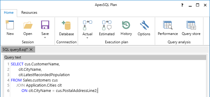
Imagine that you’ve been asked to write a query to return the population for the cities where customers are located. You think that this is an absurd request (I certainly think it’s absurd!) but yours is not to reason why, so you get busy and write something like this:
USE WideWorldImporters;
GO
SELECT cus.CustomerName,
	cit.CityName,
	cit.LatestRecordedPopulation
FROM Sales.customers cus
     JOIN Application.Cities cit
	ON cit.CityName = cus.PostalAddressLine2;
You show your boss the results, pleased that you could show the results so quickly. Your boss agrees that the results are correct, then asks you, “How’s the performance of this query?” You weren’t ready for that question, so you go back and add the statement:
SET STATISTICS IO ON;;
just before your query. You’re dismayed to see the results:
(23 row(s) affected)
Table 'Workfile'. Scan count 0, logical reads 0,
Table 'Worktable'. Scan count 0, logical reads 0,
Table 'Cities'. Scan count 1, logical reads 497,
Table 'Worktable'. Scan count 0, logical reads 0,
Table 'Customers'. Scan count 1, logical reads 40
What! Almost 500 reads to the Cities table and 40 to the Customers table, just to return 23 rows! You think that can’t be right, but a few retries yield the same results. At that point, you remember something you read about how SQL Server figures out how to get the results to a query. There’s something called an optimizer that produces an execution plan and you suspect there must be something going wrong there. The good news is, you’re right! Now, what to do about it?
Viewing the Query in ApexSQL Plan
I’ve got ApexSQL Plan, tool for visualizing and viewing SQL Server query execution plans, installed which is custom-made for situations like this. So, let’s see what we can learn about this troublesome query there. When I launch ApexSQL Plan and paste in my query, the top part of the screen looks like this:
The options in the Session and Connection sections are pretty much self-explanatory. The Execution plan section looks interesting though. Let’s start by hitting the Estimated button. After that completes, there is a lot of new information to look at:
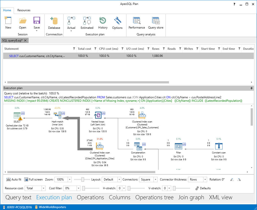
At the bottom, above the blue strip which holds the current connection information, there are a number of tab names. We started with just the “Query text”, but now the second tab, the “Execution plan”, is automatically highlighted.
Just above the tab names is a configuration section, where you can customize the display in various ways to make it easy for you to view. For now, we’ll stick with the default display.
The top section, which begins with the word Statement, is a summary of expected performance. Notice that, even though this is just an estimated plan, the estimated number of rows to be returned is already way over the 23 we know we’ll get back.
The middle section, labelled “Execution plan”, is where the action is. There’s quite a lot going on here. Each icon represents an operation that is part of the overall plan. Reading from left to right, the query is executed as a hash match between a scan of the city table’s clustered index and a nested loop of the customer table’s clustered index and other SQL Server indexes on that table. I want to draw your attention to just two items, though:

First, inside the red square, we can read that SQL Server will do a clustered index scan of the Cities table. That means it will read every row of that table looking to match the predicate in the JOIN clause of the query:
ON cit.CityName = cus.PostalAddressLine2
The reason for that scan is in the missing SQL Server index message I have highlighted. Basically it says that if there was an index on the CityName column that also included the LastReportedPopulation column, the cost of the query could be reduced by about 95%! That’s significant!. Before we change anything though, let’s actually run this query from ApexSQL Plan to see if the actual statistics match the estimates. So, I’ll click on the “Actual” button. When I do, I’m warned that my query will be run against the target server:
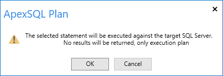
This gives me a chance to stop and think about it. Will my query affect any persistent data? (It won’t.) Will it cause such a performance impact that other users may be affected? Perhaps I should warn others that I’m about to run a sub-optimal query. Since this is just me and my laptop, I’ll go ahead and click OK.
When the query is done, the display changes to show what really happened on the server when I ran this query:
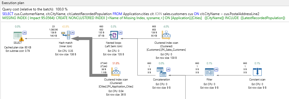
Now I can see the actual numbers and compare them to the estimated plan. In fact, ApexSQL Plan makes it easy to compare query results. If I click on the History button in the Execution plan section, I see this:
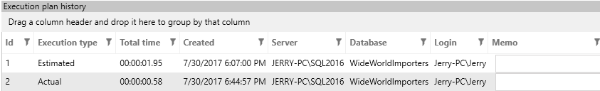
By alternately selecting the Estimated and Actual results in the history display, the view changes to match the one selected.
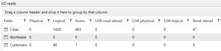
The Actual plan matches the Estimated plan quite well. The plan is still not a good one but at least we’re consistent! After running the Actual query, there is also a new tab at the bottom, I/O Reads, which in my case looks like this:
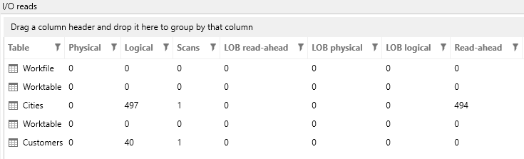
I still see a total of 537 logical reads, and two scans, plus the number of read ahead operations SQL Server did to facilitate the query. (Physical reads are zero since I’ve run this query multiple times and by this time, both tables have been cached.)The next thing to try is implement that missing index, so let’s do that!
Staying in ApexSQL Plan, I’ll open a new session and write the query to create the index:
CREATE NONCLUSTERED INDEX IX_Cities_CityName on Application.Cities (CityName)

        INCLUDE (LatestRecordedPopulation);
Running that, the new index is now in place. Now, let’s go back to the first query and get a new Actual plan. The difference is notable:
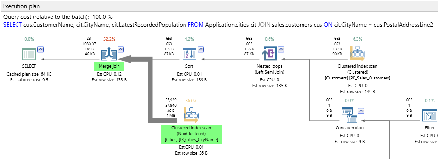
Now the plan uses a merge join instead of a hash join. That means that the two inputs must be in a certain order (alphabetically by city, in this case) and that is why there is also a sort operator to the right of the merge join. Looking at the row counts though, SQL will only have to sort 663 rows – no hardship there. Also the SQL Server index scan has changed from clustered to non-clustered. It is now using the index I just created (and the missing index message is gone). To understand why this is important, recall that a table is either a clustered index or a heap. The first execution read the clustered index – that is, the whole table; the second query just reads the new non-clustered index, which is smaller. Because of that, the I/O counts are different:
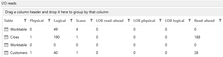
We’ve been able to trim about 260 reads from the query, which is more than 45%. A definite improvement!
If you’ve been around SQL Server for a while and seen a few execution plans, you may be wondering why the optimizer did not choose seeks against the cities table instead of an index scan as shown. Recall that the SQL Server query optimizer is a cost-based optimizer. It quickly considers a few likely plans and chooses the one with the lowest computed cost. Now maybe you think you know better! We can actually force SQL Server to do seeks if we change the query like this:
SELECT cus.CustomerName,
	   cit.CityName,
	   cit.LatestRecordedPopulation
FROM Sales.customers cus
	   JOIN Application.Cities cit WITH (FORCESEEK)
	   ON cit.CityName = cus.PostalAddressLine2;
The “WITH (FORCESEEK)” hint on the join will do just what it says. So, let’s give that a shot! This time the execution plan looks like this:
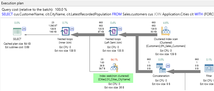
We have the Index Seek as desired, but now the main join operator is Nested Loops, which is usually the worst kind of join, since it can lead to an runtime, which is the Cartesian product of the tables being joined. Also, SQL Server spent 94.1% of its time performing index seeks! The statistics on the query show that we are worse off than before:
Now, we have many more logical reads than we started with (almost three times as many). Plus, just look at the scans on the city table! 663, or one for each row in the customer table. This goes to show that our intuition can fail us and that we should usually let the optimizer do its job!
Summary
When you have an under-performing query, there are many factors to look at. One of the most common is how SQL Server uses indexes and whether the tables in the query have the best indexing to support the query. ApexSQL Plan can really help here. You can easily try out a variety of options and compare the results of each. In this article, adding a suggested missing index reduced the i/o counts by almost half.
Before you add indexes to support any query though, you should ask yourself some questions. How often will this query be executed? How much time or I/O will be saved? Is the cost of adding and maintaining an additional index offset by the improved performance? If a query is run hundreds or thousands of times a second, usually the index is worth it. If it is an ad-hoc query run a few times a year, perhaps not.
References
- Introducing WideWorldImporters: The new SQL Server sample database
- Download Wide World Importers sample database
- Finding Missing Indexes
- Related Query Tuning Features
August 10, 2017