How to optimize SQL Server query performance – Statistics, Joins and Index Tuning

Have you ever gotten a new computer, hooked it up, and said: “this computer is blazing fast, I love it”? I have. A year from then, I was like “this computer is so slow, I need a new one”.

Performance is a big deal and this was the opening line in an article that was written on How to optimize SQL Server query performance. The initial article shows not only how to design queries with the performance in mind, but also shows how to find slow performance queries and how to fix the bottlenecks of those queries. I’d highly recommend reading the above article first because this one would give a lot more meaning but also because it’s an appendix to this topic.

Before we continue further, here’s a quick recap of the covered subjects and their main goals:

• Query optimization overview – In this part, we got familiar with what query plans are all about. This part explained in detail how query plans help SQL Server in finding the best possible and efficient path to the data and what happens when a query is submitted to SQL Server including steps that it goes through to find those routes. Furthermore, we also covered statistics and how they help the Query Optimizer to build the most efficient plan so that SQL Server can find the best way to fetch data. We also mentioned a few tips and tricks (guidelines) on how to be proactive in designing queries with the performance in mind to ensure that our queries are going to perform well right out the gate.
• Working with query plans – Here we jumped over to a tool called ApexSQL Plan to get familiar with query plans and understand how to “decipher” them which will ultimately help us find the bottlenecks in slow performance queries. We mentioned statistics again, but this time we’ll also show where they’re stored in SQL Server and how to view them. Furthermore, these statistics can be maintained and kept up-to-date to ensure that the Query Optimizer will create the best guesses when fetching data. We also covered examples of different use case scenarios on how SQL Server is accessing data using full table scan vs full index scan vs index seek, etc.
• Optimizing query performance – In the last part, we put some of those guidelines from previous sections into use. We took a poorly designed query and applied design techniques to practice by writing it the right way. In the end, we wrapped things up with best practices and some guidelines. We barely touched a few topics that play a big role when it comes to querying performance and the purpose of this article is to get familiar with those topics in detail and put them to practice with some examples.

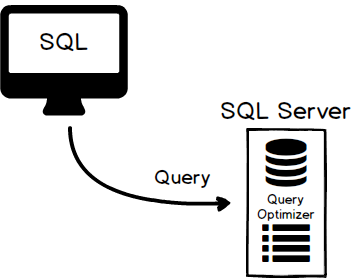
So, let’s first summarize what’s happening under the hood when we hit that execution button. Think of a query/execution plan as just a map. It’s a map that SQL Server is drawing of the most efficient path to the data. When SQL Server accepts a query coming from either an application or directly from a user, it passes it to the Query Optimizer which will then create a query/execution plan:

This execution plan is just SQL Server method to access data stored in data pages on disk. These query plans require resources to create and therefore SQL Server will cache them:

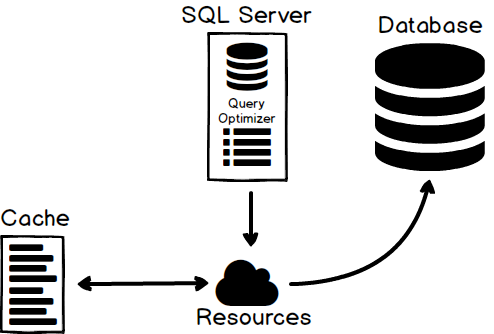
The next time a query comes in and has a similar Where clause or path to the data, SQL Server will reuse the query plan for performance game. There are of course aging algorithms that will remove old query plans from the cache, but this is internal stuff and, as always, SQL Server does a great job at managing it.

Statistics

So, we already said that statistics are important because they help the Query Optimizer. We also briefly described that statistics hold information about columns the Query Optimizer uses to generate query plans. You might be wondering how exactly statistics help the Query Optimizer to make its best guesses when accessing data? Here’s a good analogy to answer this question. If you ever planned a party, most of the time when people send invitations they’ll say, “please RSVP” which basically means “please respond” whether or not they plan to attend the party. They do this so they can plan accordingly: how much food to order, how many drinks to get, etc. because this allows them to have a better estimate of all those stuff they need so they don’t get too many or too little and that’s exactly what statistics do. The more up-to-date statistics are the better decisions will Query Optimizer create on how to execute a query and find data the efficient way.

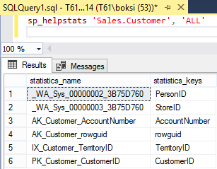
The statistics are created on indexes and columns. So, the first thing we can do is to run the sp_helpstats stored procedure that returns statistics information about columns and indexes on the specified table. Run the query below passing the name of your table and the “ALL” parameter that will give us both the indexes and statistics that are generated for the specified table:

sp_helpstats[ @objname = ] 'object_name'   
     [ , [ @results = ] 'value' ]

Executing this command will return all auto-generated and managed statistics and indexes by SQL Server:

This is as basic as it gets. However, we can run DBCC SHOW_STATISTICS command to displays current query optimization statistics for a specific table or indexed view. Again, passing a name of your table and a name of statistics:

DBCC SHOW_STATISTICS ( table_or_indexed_view_name , target )

In this case, we’re going to look at the primary key (PK_Customer_CustomerID) of the CustomerID which is clustered index that will show us all statistics information:

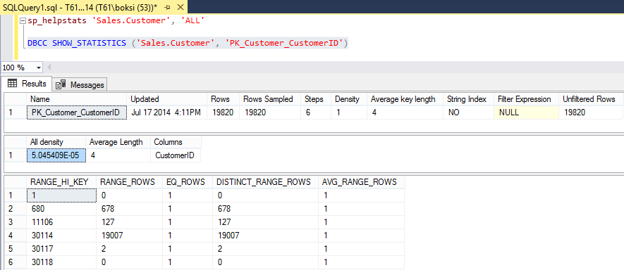
The returned table information in the result set shows various useful information like a total number of rows in the table or indexed view when the statistics were last updated, an average number of bytes per value for all the key columns in the statistics object, a histogram with the distribution of values in the first key column of the statistics object, etc. The point is all those stats are going to help the Query Optimizer in making the best decision to create the best execution plan possible.

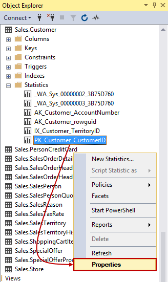
This exact information is also available from Object Explorer. If we navigate to a table in a database, there should be a Statistics folder under it which holds the data we previously saw in the result set. To do this, right-click a statistic and choose Properties at the bottom of the context menu:

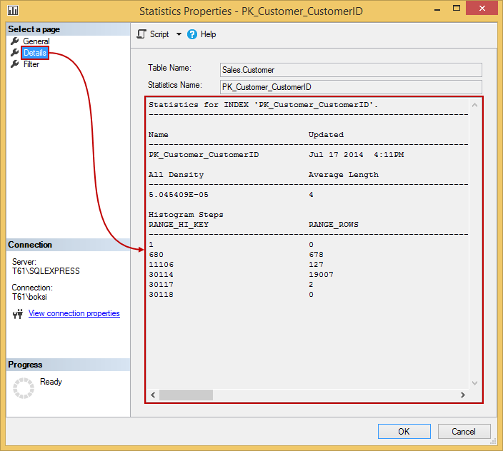
If we switch over to Details page in the top left corner, we’ll see the exact same data that we were just looking at:

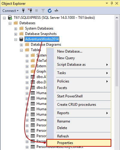
We did mention that SQL Server manages to update of these statistics automatically and you can verify this setting by going to your database in Object Explorer, right-clicking it and choosing the Properties command at the bottom of the context menu:

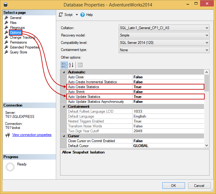
If we switch over to Options page in the top left corner, you should see under the Automatic rules two items: Auto Create Statistics and Auto Update Statistics options set to True:

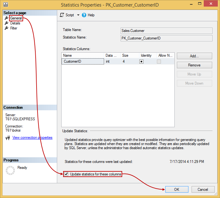
Probably a good idea to leave those enabled unless you want full control over statistics creation and updating. However, if e.g. there is a reason to update them manually we can just go to statistic’s properties and under the General page, you’ll find the Update statistics for these columns option. Here’s also the information on when the statistics were last updated. Select this option and hit the OK button to automatically do an update on the spot:

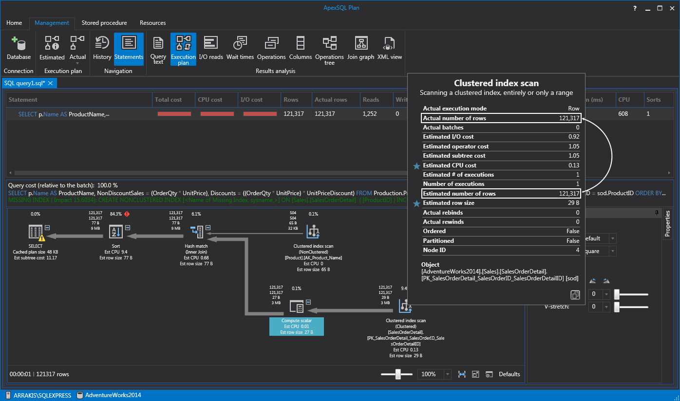
The Query Optimizer determines when statistics might be out-of-date and then updates them when needed for a query plan. If you’re wondering how we can tell if the statistics are getting stalled, well we can usually see this by looking at the execution plan. How? In most situations just by looking at the estimated rows and actual rows. If we hold the mouse over an operation it will bring up the tooltip in which we can see if there’s a big gap between the Actual number of rows and Estimated number of rows then we know that statistics need to be updated. In the case below both numbers are the same which means the statistics are up-to-date, so update those manually only if the numbers are wildly off:

Joins

In the initial article, we covered different types of scans and indexes. Often, we write complex queries with multiple tables involved, joining data from different tables. Well, this is where SQL Server internally has three different ways to tie data from multiple tables together joining them. We know it, in the T-SQL world, as the Join statement but SQL Server under the hood has many ways that it can join data together and it’s always going to choose the best one. I just want to show you how they look like in execution plans and because it’s good to know in general how SQL Server internally brings data together.

Let’s start off by writing a simple Join statement of two tables. We can actually force the Query Optimizer to use a specific type of join when it joins tables together. This can be done by using either loop, hash, or merge options that enforces a particular join between two or more tables. The following example uses the AdventureWorks2014 database:

SELECT p.ProductID, p.Name, p.ListPrice, p.Style FROM Production.Product p
JOIN Sales.SalesOrderDetail sod ON p.ProductID = sod.ProductID
OPTION(LOOP JOIN)

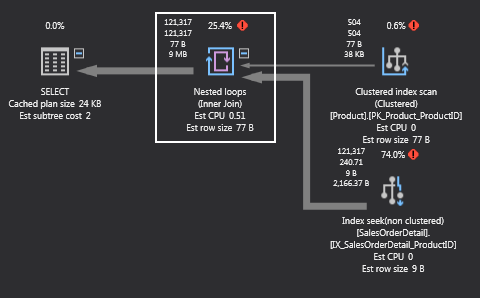
If we look at the execution plan of the above query in ApexSQL Plan, we’ll see that SQL Server is doing a loop join. What this loop basically does is for each row in the outer input, it’s scanning the inner input and if it finds a match it’s going to output it into results:

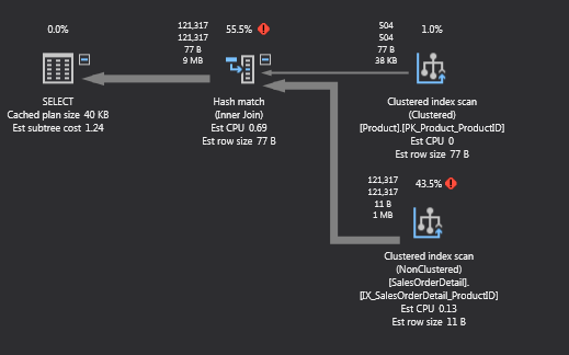
If this is the best way to join data? Well, let’s execute the same query but without forcing the type of join. To do this, just remove the options parameter. This time the Query Optimizer chose the merge join:

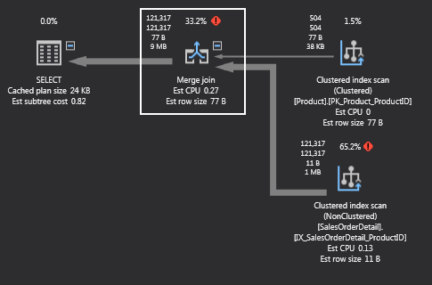
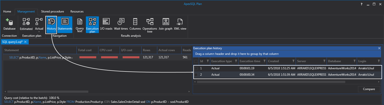
I’m sure that some will say, “Hey, we just went from 25.4% to 33.2%. How is that good”. Well, that’s not the point. Similar to the rules for index scans vs index seeks, some rules apply in general but do not necessarily mean that it will always be the most efficient way. Also, most of the cost will come from merge join because it has to sort the data. Bear with me, we can prove this by hitting the History tab from the main menu to view the execution plans for both queries. If we look at the Execution time column, note the time counter is 1.19 when we forced the loop join and less when the Query Optimizer chose merge join:

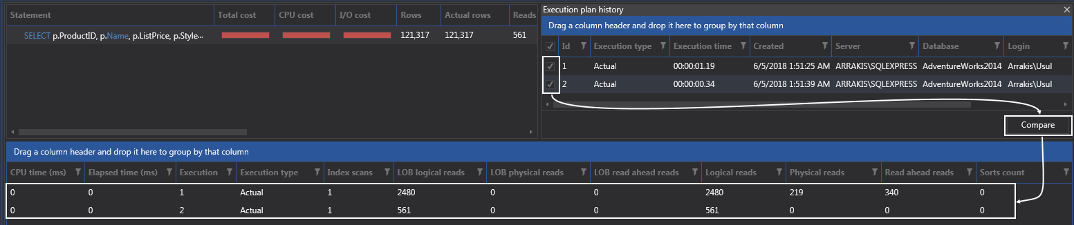
Furthermore, we can also check both plans and hit the Compare button to see additional stats and from this example, we can see that merge join is performing much better just by looking at the reads columns:

Let’s also see what a hash join does by forcing the execution plan to use it:

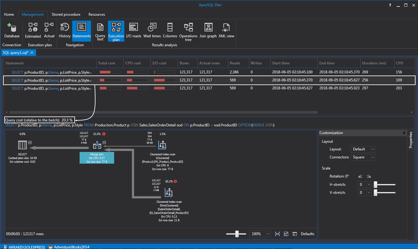
Numbers can be confusing sometimes. What I like to do is put all three joins in the same query text and look at the execution plan:

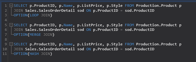
What we get in the execution plan when placing multiple statements is an overview of total query cost relative to the batch. In this case, if we select the statement with the merge join, which is also the type of join SQL Server will choose by default, we can see below in the execution plan that the total query cost is 20.3%:

If we switch over to other two, we can see that the loop join took 46.6% and the hash join took 33.3%:

So, the hash join is for large amounts of data. It’s really the work course that SQL Server is going to use for things like table scans or index scans, anything that isn’t a seek, also in cases when it’s a seek but still, it’s pulling a large amount of data.

Now, the general rule of thumb is nested loops are good for small amount of data. The SQL Server will most likely choose this type of join when there’s not a lot of data to work with. You’ll see the merge join with a medium amount of data, and the hash joins with a large amount of data. If the queries are covered with indexes, SQL Server will work with less amount of data and this is where loop joins are most likely to be seen. On the other hand, if you’re missing indexes, SQL Server will work with a large amount of data (table scans) and you’ll probably see hash joins or at least merge joins.

Index Tuning Wizard

Back to indexes, remember that we should revisit them often. On a database with a large number of objects this sound like mission impossible. Not really. Let’s take a look at one tool, part of SQL Server, that’s called Index Tuning Wizard which can help us with this stuff. Remember that the biggest single thing we can do in our databases performance-wise is have a good indexing strategy.

So, let’s get familiar with this Index Tuning Wizard and see what we can do with it. This tool can be used when developing an application, database, or query. The first thing we should do is to set up a workload. This is done by running a query against your database and trapping the results. Then we can send these results to Index Tuning Wizard which will tell us, based on the query itself and results, what should be indexed and covered by statistics and give us recommendations in general.

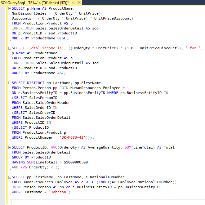
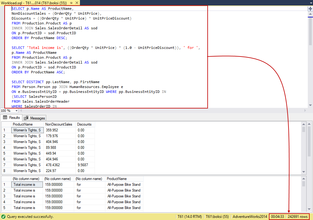
A workload is just a set of T-SQL statements that execute against a database that we want to tune. So, next step is to either type our T-SQL script into the Query Editor or use e.g. existing stored procedures (turn them into a workload). To simplify this example, we’re going to use a series of the most used Select statements that are hitting our database. As shown below, this is just five frequently used Select statements in one query:

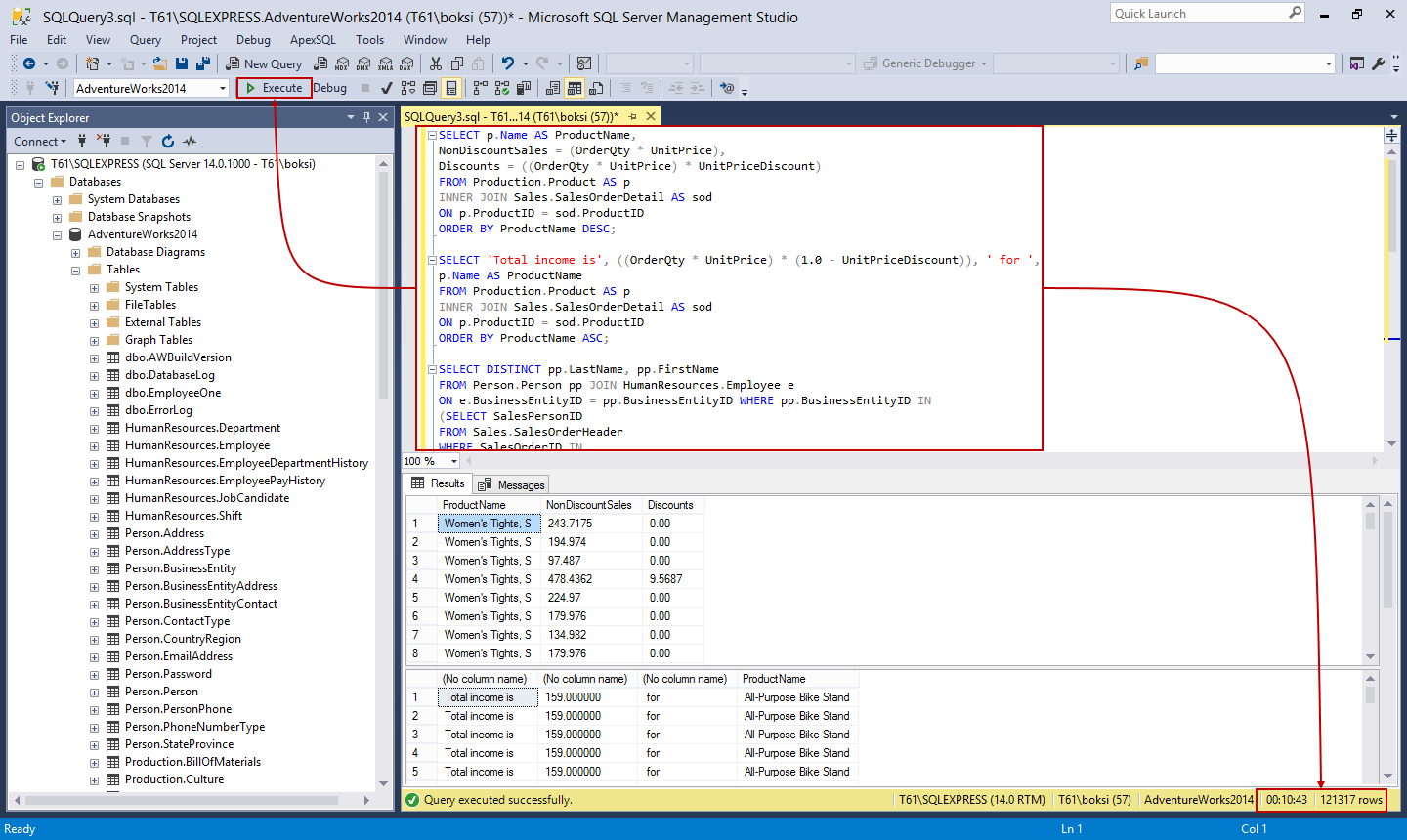
It’s always a good idea to execute the batch just to verify that the query is valid and that the result set is without warning or errors. Also, after a successful execution, the status bar of SSMS will present the number of rows returned and the total duration time. As we can see from this example, the whole process took over ten minutes and returned 242K+ number of rows which is a pretty good workload:

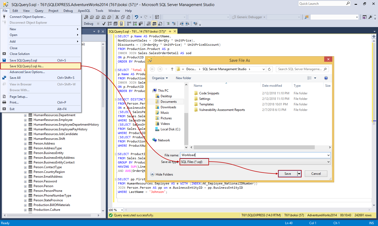
All we should do now is save the file with a .sql extension:

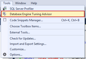
Next, on the SQL Server Management Studio Tools menu, click Database Engine Tuning Advisor:

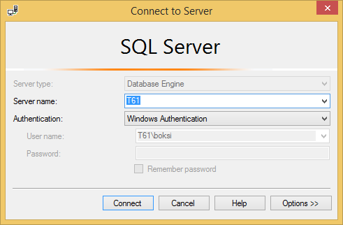
This will pop-up the Connect to Server dialog, so leave everything as it is or make the appropriate changes and hit the Connect button to continue:

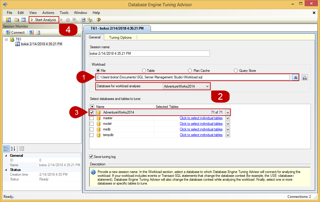
In the next window, we need to set a few things up before we can continue further:

1. Browse for the workload file that was previously created
2. Select the appropriate database for workload analysis
3. Select the appropriate database and tables to tune
4. Click the Start Analysis button to start the next tuning step

The Progress bar shows information about actions taken and their status:

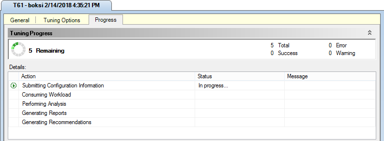
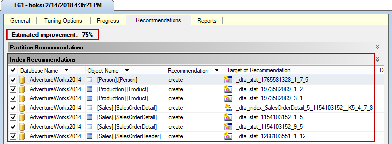
It will go thru the steps of tuning five times and once it’s done it will move on to next step (Recommendations tab). This step might take a while, but once it’s done, a list of index recommendations will be shown. There’s also estimated improvement number (75% in this case) which is informative in its way. Is it true? Well, let’s finish the optimization and check the results later:

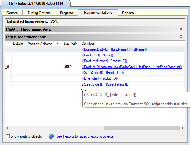
If we scroll horizontally to the right, there’s a column called Definition under which there’s a preview T-SQL code for creating those missing indexes and statistics:

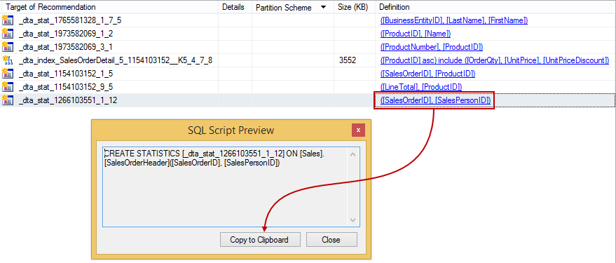
Clicking on a link from the Definitions list will open the SQL Script Preview window showing the T-SQL script for creating missing indexes and statistics which can be copied to the clipboard and used later:

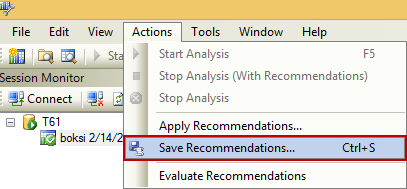
Instead of copying each script one-by-one to the clipboard (when the list is long), we can save all the recommendations by clicking the Save Recommendations command in the Actions menu:

Once it’s done, this newly created script can be executed against the targeted database:

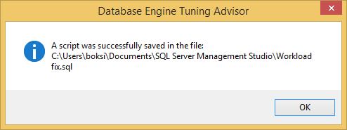
Go back to SSMS, open the script and execute it. There should be a message that the command completed successfully:

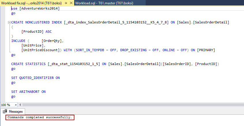
Most of us would not be able to figure it out exactly how to create these best possible indexes and statistics, but this tool makes our lives easier.

Back to the estimated improvement number… how did creating the indexes and statistics improved overall performance? Good. Running the same heavy query, the execution time went down almost by a half.

Bear in mind that the number represented in the Database Engine Tuning Advisor is just an estimation. The results might vary but overall there should be an improvement.

One last thing, also getting familiar with Dynamic Management Views (DMV) can also help us find slow performing queries. This tool can be used to find poor or long time running queries. It is actually just a collection of views and functions that can be run to find information about SQL Server. These views and functions return data about what is going on in SQL Server. There’s a lot of docs on Microsoft official site and they’re also categorized nicely, so it’s highly recommended to check out online books and find out more about DMVs.

Here are the two quick ones that can be used in the real word on any SQL Server:

-- Return top 10 longest running queries
SELECT TOP 10 qs.total_elapsed_time / qs.execution_count / 1000000.0 AS AverageSeconds,
              qs.total_elapsed_time / 1000000.0 AS TotalSeconds,
              qt.text AS Query,
              DB_NAME(qt.dbid) AS DatabaseName
FROM sys.dm_exec_query_stats qs
     CROSS APPLY sys.dm_exec_sql_text(qs.sql_handle) AS qt
     LEFT OUTER JOIN sys.objects o ON qt.objectid = o.object_id
ORDER BY AverageSeconds DESC;

The above query will return the top 10 longest running queries in a database. All this query does is basically just running the sys.dm_exec_query_stats view that returns information about a query that is sitting in a database specified in the Select statement and then cross apply it to a table value function passing the handle (which is a column from a view) which will give us the actual query that was executed.

The query below will return the top ten expensive queries in term of input/output (disk read operations):

-- Return top 10 most expensive queries
SELECT TOP 10(total_logical_reads + total_logical_writes) / qs.execution_count AS AverageIO,
             (total_logical_reads + total_logical_writes) AS TotalIO,
             qt.text AS Query,
             o.name AS ObjectName,
             DB_NAME(qt.dbid) AS DatabaseName
FROM sys.dm_exec_query_stats qs
     CROSS APPLY sys.dm_exec_sql_text(qs.sql_handle) AS qt
     LEFT OUTER JOIN sys.objects o ON qt.objectid = o.object_id
ORDER BY AverageIO DESC;

Neither of them will return any data in this case because there’s no real activity in the environment (SQL Server) set up for this article but use these on a big server that has a lot of activity and the results set will be filled with data.

I’d wrap things up by saying one last tip and that is to also get familiar with SQL Server Profiler. With this tool, we can set up a trace against a server or database and basically trap all the statements coming into either server or database. Furthermore, this tool allows us to see exactly what is hitting our server, what data is being passed and parameters, logins, and logouts, etc. It also integrates with the Index Tuning Wizard, we saw it when we created the workload. Once you get the hang on all these tools and you combine them with the executions plans, the query troubleshooting will become much easier.

I hope these two articles have been informative for you and I thank you for reading.

• How to optimize SQL Server query performance
• How to optimize SQL Server query performance – Statistics, Joins and Index Tuning

Useful links

• Statistics
• How to: Create Workloads
• Start and Use the Database Engine Tuning Advisor
• System Dynamic Management Views
• SQL Server Profiler